Plot an imat_fn in a special GUI that provides extended functionality.
g=uiplot(f)
uiplot(f,g,...)
g=uiplot(f,z)
UIPLOT provides a convenient graphical user interface for plotting imat_fn. You can plot functions individually, overlaid, or stacked. Plots are overlaid according to ordinate data type. You can control the plot style through the “Mode” pulldown in the Plot panel at the bottom left of the UIPLOT window. A context menu (right-click over the plot) allows you to window, apply tags,and change the overall plot appearance.
F is an imat_fn (or fcn). You can pass in more than one imat_fn variable. Z is an optional input containing an imat_filt, or a structure with the fields .name and .index. The .index field must contain valid numeric indices into F. The .name field must contain a string. This is the filter name that will be displayed in the UIPLOT GUI. These optional input arguments are not available when running standalone UIPLOT.
UIPLOT also provides the ability to create and apply templates to plots. Once a plot is configured as desired, all subsequent plots can have the same appearance. The settings can be saved and loaded for use during a different session.
All plots can be exported to image files or shown as a slideshow. A command window allows standard MATLAB commands to be used to format the plots.
If G is requested, UIPLOT blocks input on the command window. By default, however, UIPLOT is non-blocking, meaning control is returned immediately to the MATLAB prompt.
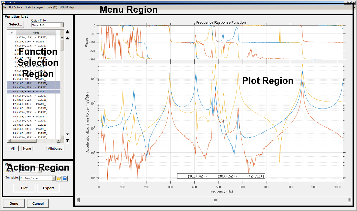
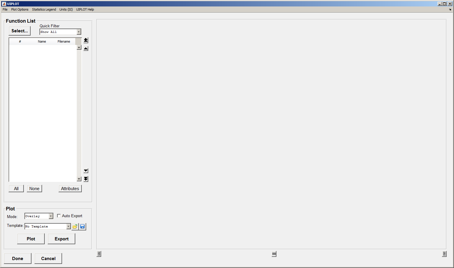
In MATLAB, you can start UIPLOT by typing uiplot at the MATLAB command prompt. If you are running the standalone executable, you can start UIPLOT through Windows Start -> Programs menus. This will bring up the main interface, shown in Figure 1.
Figure 1: UIPLOT Main Interface
The main interface of UIPLOT has four distinct functional areas, which are highlighted in Figure 2.
Figure 2: UIPLOT interface regions.
The Plot Region contains the axes where all plots will be created. The set of plots currently displayed is considered a slide. As mentioned previously, if the requested slide will contain more axes than can be displayed, they will overflow onto addition slides and can be navigated using the buttons at the bottom of the Plot Region. The units pulldown allows you to change the plot display units. This only affects the plot; it will not modify the data returned by UIPLOT.
The File menu in the Menu Region controls the most basic functions of UIPLOT.
| Load File | Functions are loaded by selecting the Load File menu item and subsequently selecting an appropriate file from the Open File dialog box. The loaded functions will appear in the function list in the Function Region at the left side of the interface. Supported file formats available to load are FCN, AFU, ATI, PCH (NASTRAN) and .vra_xyout (Vibrata). |
| Load Workspace | The Load Workspace menu item allows you to select variables from the base workspace to load into UIPLOT. The loaded functions will appear in the function list in the Function Region at the left side of the interface. Supported function types are IMAT_FN and FCN. |
| Plot |
The Plot menu item will plot the selected functions in the Plot Region. The plot preferences are set using the controls in the Action Region. After any change has been made to the plot options, the Plot button must be pressed again to plot the functions with the new options. Plots can be overlaid by type, stacked, or cycled. This is controlled by the Mode pulldown. The Overlay by Type option will plot the functions grouped by ordinate data type. The Stack option will plot each function individually, with the total number on each slide controlled by the Plots Per Page option in the Plot Options menu. The Cycle option will plot one function on a slide in the Plot Region. In all cases, if the plots do not fit onto one slide, the navigation buttons at the bottom of the plot will be activated and can be used to navigate the slides. The current slide and total number of slides will appear at the lower left of the Plot Region. By default, each plot also will contain a legend describing the lines of the plot. This option can be toggled on or off from the Plot Action menu. |
| Save File | The Save File menu item will save any selected functions in the Function Region to a new file. A number of output formats are supported, including I-deas Associated Data Files (AFU or ATI), Vibrata FCN files (.fcn), Universal files (.unv), Comma-separated variable files (.csv), and NASTRAN TABLED1. |
| Save Workspace | The Save Workspace menu item will save any selected functions in the Function Region to the base workspace. |
| Export | The Export menu item will save the current slide to an image file. The available formats are BMP, EMF, PNG, PS, or TIFF. The format for output can be changed by selecting the format on the dialog box. |
The Action Region controls how UIPLOT creates each slide.
| Plot | The Plot menu item will plot the selected functions in the Plot Region. The plot preferences are set using the controls in the Action Region. After any change has been made to the plot options, the Plot button must be pressed again to plot the functions with the new options. Plots can be overlaid by type, stacked, or cycled. This is controlled by the Mode pulldown. The Overlay by Type option will plot the functions grouped by ordinate data type. The Stack option will plot each function individually, with the total number on each slide controlled by the Plots Per Page option in the Plot Options menu. The Cycle option will plot one function on a slide in the Plot Region. In all cases, if the plots do not fit onto one slide, the navigation buttons at the bottom of the plot will be activated and can be used to navigate the slides. The current slide and total number of slides will appear at the lower left of the Plot Region. By default, each plot also will contain a legend describing the lines of the plot. This option can be toggled on or off from the Plot Action menu. |
| Mode | The Mode pulldown controls whether the plot will be overlaid by type, stacked or cycled. See the text for Plot for more information. |
| Auto Export | If enabled, all plots subsequently generated by the Plot button will be automatically exported to a file. A dialog box will first appear however, requesting a base name for the outputted files. The format is controlled by the Save As Type pulldown on the dialog box. |
| Template | All loaded templates will appear in the Template pulldown. To use a template, select it from the list and press Plot. To plot with out a template, select No Template as the template. |
| Open Template | The Open Template button has a folder icon on it. This button opens an existing template file and adds it to the list of available templates. |
| Save Template | The Save Template button has a disk icon on it. This button saves the settings of the current slide to a file. A file dialog will appear where the name and location of the file can be entered. |
The Function Selection Region displays the functions that have been loaded into UIPLOT and provides methods for selecting specific functions. The function number, name, and corresponding filename are shown in the table. The single arrow buttons to the right of the list will move the current selection in the function list up or down. The double arrow buttons will jump the current selection to the very top or bottom of the list.
| All | The All button selects all of the functions in the function list box. |
| None | The None button deselects all of the functions in the function list box. |
| Select... |
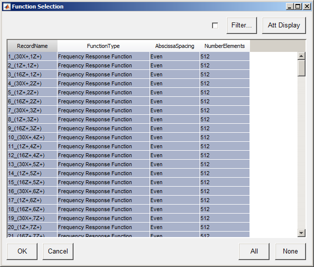
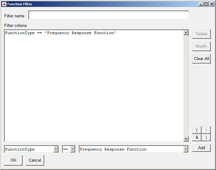
The Select... button is used to create a custom selection of functions, and selecting it will open the Filter Functions window, seen in Figure 4. This window displays all loaded functions, and provides pulldown menus for displaying function attributes. A custom filter can be created by selecting the Filter... button at the top-right of the window. This will bring up the form seen in Figure 5. The filter generated by Select... will then be applied to the functions listed on the main UIPLOT window. To select functions using a custom filter, combine the attribute, attribute value, and operator at the bottom of the form as desired, and press the Add button. This will add the filter to the list. Multiple filters can be combined to form a single filter. Once the desired combination of filters has been created, press the OK button to return to the Filter Functions window. The function list in this window should now display the list of functions after the new filter has been applied. Select OK to return to the main interface. |
| Quick Filter | The Quick Filter pulldown is used to quickly apply filters to the full function list. Standard filters are Drive Point and Reciprocity. The <<Select Button>> item is used to return to the selection that was made using Select... |
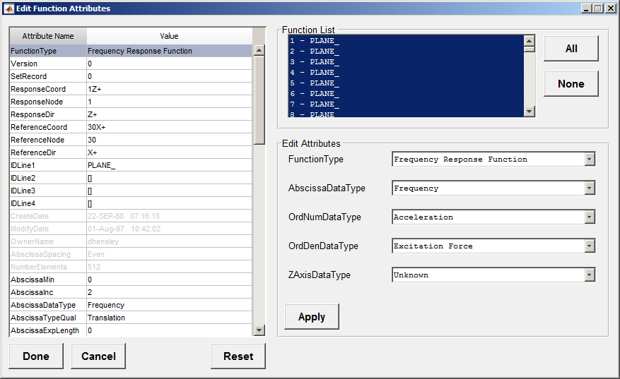
| Attributes | The Attributes button will launch the Edit Function Attributes window seen in Figure 3, with the selected functions from the Function Region preloaded into the interface. From this window, any editable function attribute can be changed. The functions will appear in the Function List section of the window, with all the attributes listed in the table on the left side of the window. Selecting an attribute from the table will refresh the Edit Attributes section, where the attributes can be edited. To set the changes, press the Set button and the changes will be reflected in the table. The Done button on this form will save the changes made, and return to UIPLOT. The Cancel button will also close the window and return to UIPLOT without saving anychanges that were made to the attributes. The Reset button will reset the functions to their state when the Edit Function Attributes window was opened, but will keep the window open so new changes can be made. |
Figure 3: Edit Function Attributes Window
Figure 4: Filter Functions Window
Figure 5: New Filter Window
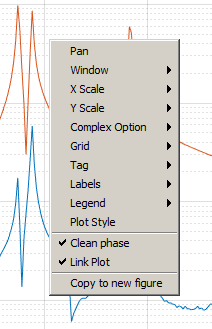
The contextual menu, which controls many aspects of the plot appearance, can be activated by right-clicking on any plot in the Plot Region, as seen in Figure 6. The following options are available:
| Window | None | When selected, axis limits will be controlled by MATLAB. |
| Tight | When selected, axis limits will be adjusted to exactly envelope the data plotted. | |
| Pick X | When selected, X limits will be defined by manually picking them from the plot. | |
| Pick Y | When selected, Y limits will be defined by manually picking them from the plot. | |
| Pick XY | When selected, both X and Y limits will be defined by manually picking them from the plot. | |
| Key in X | When selected, X limits will be defined by manually typing them in. | |
| Key in Y | When selected, Y limits will be defined by manually typing them in. |
| XScale | Default | When selected, the X axis will be set to its default, which varies by Function Type. |
| Linear | When selected, the X axis will be displayed on a linear scale. | |
| Log | When selected, the X axis will be displayed on a logarithmic (base 10) scale. |
| Y Scale | Default | When selected, the Y axis will be set to its default, which varies by Function Type. |
| Linear | When selected, the Y axis will be displayed on a linear scale. | |
| Log | When selected, the Y axis will be displayed on a logarithmic (base 10) scale. |
| Complex Option | Default | When selected, the plot format will be set to its default. |
| Modulus + Phase | When selected, the plot will be displayed in two axes. The lower axis displays the modulus (magnitude), and the upper axis displays the phase. | |
| Modulus | When selected, the plot will show just the modulus (magnitude). | |
| Phase | When selected, the plot will show just the phase. | |
| Real + Imaginary | When selected, the plot will be displayed in two axes. The lower axis displays the real part of the functions, and the upper axis displays the imaginary part. | |
| Real | When selected, the plot will display the real portion of the functions. | |
| Imaginary | When selected, the plot will display the imaginary portion of the functions. | |
| Nyquist | When selected, the plot will converted into a Nyquist plot, with the real part of the function plotted on the X axis, and the imaginary part plotted on the Y axis. |
| Grid | X and Y | When selected, grid lines will be applied in both the X and Y directions. |
| X only | When selected, grid lines will only be applied in the X direction. | |
| Y only | When selected, grid lines will only be applied in the Y direction. | |
| None | When selected, no grid lines will be applied to the plot. |
| Tag | Tag on Grid | When selected, the Tag on Grid option will activate crosshairs to tag any grid point on a plot. |
| Tag on Data | When selected, the Tag on Data option will activate crosshairs to tag any data point on a plot. Any click on the plot will tag the nearest data point. | |
| Tag X | When tags are applied, only the X coordinate will be tagged. | |
| Tag Y | When tags are applied, only the Y coordinate will be tagged. | |
| Tag X and Y | When tags are applied, both the X and Y coordinate will be tagged. | |
| Delete Tags | When selected, all tags on the plot will be deleted. | |
| Cursor | The cursor toggle provides a convenient vertical line to assist in tagging. |
| Labels | X Label | Changes the X Label of the plot. If the plot is two axes, the X Label always appears on the lower plot. |
| Y Label | Changes the Y Label of the axes clicked. | |
| Title | Changes the Title of the plot. The title always appears on the upper-most axes. | |
| X Label Font | Brings up a GUI that lets you select the X Label font. | |
| Y Label Font | Brings up a GUI that lets you select the Y Label font. | |
| Title Font | Brings up a GUI that lets you select the Title font. | |
| Reset | Resets the X Label, Y Label, and Title to their default values. The default values are determined by what type of data is plotted. |
| Legend | Show Legend | Toggles whether the legend is shown on the figure. |
| Default | Sets the legend to label the plotted lines with the default labels. | |
| IDLine1 | Sets the legend to label the plotted lines with their IDLine1 value. | |
| IDLine2 | Sets the legend to label the plotted lines with their IDLine2 value. | |
| IDLine3 | Sets the legend to label the plotted lines with their IDLine3 value. | |
| IDLine4 | Sets the legend to label the plotted lines with their IDLine4 value. | |
| Ref/Res | Sets the legend to label the plotted lines with their ReferenceCoord and ResponseCoord values. | |
| RMS | Sets the legend to label the plotted lines with their RMS value. | |
| MAX | Sets the legend to label the plotted lines with their maximum value. | |
| MEAN | Sets the legend to label the plotted lines with their mean value. | |
| MIN | Sets the legend to label the plotted lines with their minimum value. | |
| Custom | Sets the legend to use the custom text specified. | |
| Font... | Sets the legend font properties. | |
| Location | This contains a submenu that controls the location of the legend. | |
| Interpreter | This contains a submenu that controls the interpreter to be used for the legend text. | |
| Orientation | This contains a submenu that controls the orientation of the legend. | |
| Items Per Plot | This controls the maximum number of lines that will be included in the legend. |
| Plot Style | This brings up the Plot Style window where plotted functions can be formatted individually. |
| Clean Phase | If enabled, points where the phase differs by more than 270 degrees from the previous point will not be displayed. This option is enabled by default. |
| Link Plot | Link all of the plots on this figure. |
| Copy to new figure | Copy the displayed plot to a new figure window. This can be useful for exporting the plot. |
Figure 6: Contextual Menu
The Plot Options menu at the top of UIPLOT is the location of numerous references and actions for controlling UIPLOT.
| Plot Options | Legend | Opens another menu, where you can select which attribute gets displayed in the plot legend. The default is to display the reference and response coordinate. You can also specify how many legends to display per plot. |
| Plots Per Page | Controls the maximum number of plots that will appear on one slide. When selected, a dialog box will appear where the new setting can be input. The menu text will be updated to reflect the current setting. | |
| Link All Axes | This toggle links the axes of a multi-axes plot together. By default, this is turned on for all plots. Toggling this will change the setting for all plots on the current slide. | |
| Link All Plots | This toggle links multiple plots on a single slide together. If toggled, whenever a plot updates, all plots on the slide will be updated identically. | |
| Grouping | This option controls how plots are grouped for stacked and cycled plots. By default, the plots are not grouped. Optionally, they can be grouped by reference or response coordinate. | |
| Slideshow | When enabled, all plots which result in multiple slides will automatically cycle. The time between the display of each slide is controlled through the Slideshow Interval option under the same submenu. The slide show can be looped by enabling the Loop option. A slideshow can be stopped by pushing the stop button at the bottom of the Plot Region. | |
| Scale Factor | Apply a static scale factor to the plots, regardless of units. Any scalar real or complex value may be entered. When a scale factor is applied to the plots, a notation will be appended to the plot title ("<Scaled by ###>") unless you have specified a custom title. An asterisk ("*") also appears in front of the displayed statistical quantities in the Statistics Legend. You must hit Plot to apply the scale factor. | |
| Copy plots to new figures | Copy the individual plots displayed into new figures. This is equivalent to exercising the "Copy to new figure" context menu item in each plot. | |
| Copy to clipboard (bitmap) | Copy the currently displayed plot to the clipboard as a bitmap (raster image). | |
| Copy to clipboard (meta) | Copy the currently displayed plot to the clipboard as a metafile (vector image). This option is only available on Windows. |
The Statistics Legend menu at the top of UIPLOT allows you to toggle the display of statistical quantities to the right of the displayed function plots.
| Statistics Legend | Enable | When activated, a secondary legend will be added to the right of the plot which documents the statistics of the plot. The available statistics are Maximum, Minimum, Mean, and RMS. By default, they are all enabled, but can be toggled on or off through the same menu. |
| Interpolation Type | Select the interpolation type for RMS and Zero Crossing Rate calculations. Valid choices are Default, LinLin, LinLog, LogLin, and LogLog. If Default is selected, LinLin will be used for imat_fn and the value for the InterpolationType property for each function will be used for fcn. | |
| Max | The maximum ordinate value on the plot. | |
| Min | The minimum ordinate value on the plot. | |
| Mean | The mean ordinate value on the plot. | |
| RMS | The root mean square (RMS) ordinate value on the plot. | |
| ZUXR | Zero up crossing rate. |
The Units menu at the top of UIPLOT allows you to change the current units system in which the plotted functions are displayed. You must hit Plot to update the display.
The UIPLOT Help menu at the top of UIPLOT provides a way to display the UIPLOT documentation.
| UIPLOT Help | When activated, a secondary legend will be added to the right of the plot which documents the statistics of the plot. The available statistics are Maximum, Minimum, Mean, and RMS. By default, they are all enabled, but can be toggled on or off through the same menu. | |
| Report Bug/Request Feature | Opens a browser window to TIER, ATA's issue tracking website. | |
| IMAT Website | Opens a browser window to the IMAT website. | |
| RMS | Opens a browser window to the UIPLOT documentation (this page). |
UIPLOT also offers a host of other features. The slideshow feature can be accessed through Plot Options -> Slideshow. When enabled, all plots which result in multiple slides will automatically cycle. The time between the display of each slide is controlled through the Slideshow Interval option under the same submenu. The slide show can be looped by enabling the Loop option. A slideshow can be stopped by pushing the stop button at the bottom of the Plot Region.
The statistical legend can be enabled by navigating to Options -> Statistical Legend -> Enable. When activated, a secondary legend will be added to the right of the plot which documents the statistics of the plot. The available statistics are Maximum, Minimum, Mean, and RMS. By default, they are all enabled, but can be toggled on or off through the same menu.
The auto export feature toggle found in the plot panel. It works exactly like the Export button discussed earlier; however, when activated, it will automatically export all slides generated when the Plot button is pressed. The user will be prompted by a file dialog to provide a base name for the image files. The extension of the file will determine the format of the output.