SPL Module

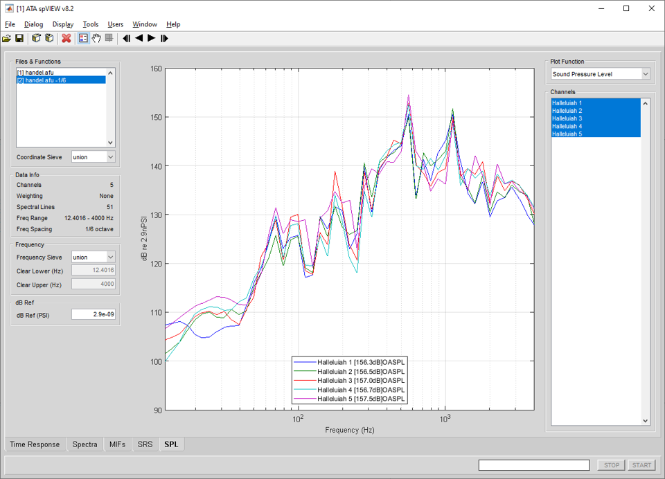
In the SPL module, frequency-domain spectra, auto-spectra, and power spectral density (PSD) functions with a data type of pressure or sound pressure are read into spVIEW and plotted as sound pressure level. Information about the selected datasets and the channels in the Coordinate Sieve is displayed in the Data Info panel.

Sound pressure level is computed as a function of frequency as

,

where f_k denotes the frequency of the spectral line and P_ref is the reference sound pressure defined for the IMAT units system.

In addition to the standard measurement function types, “SPL functions” written from the SPL Module also can be read and plotted. An “SPL function” has the following attributes:

For a function with these attributes, the ordinate SPL values (in dB) are not affected by units system conversion on read or write and the default y-label is overridden by the ordinate axis label and ordinate units label.

Selecting a plotted line with the mouse pointer and holding down the middle button will highlight that line and its corresponding entry in the plot legend and display the name from the legend in the message line at the bottom of the window. Selecting an entry in the plot legend with the middle mouse button will toggle highlighting of the corresponding line in the plot axes.

Frequency : Frequency Sieve – When multiple datasets are selected in the Files & Functions list, the Frequency Sieve determines the frequency range for plotting. The Frequency Sieve can be union or intersection, which sieves the frequency ranges of the selected datasets as set operator nomenclature implies, or manual, which allows the frequency range to be specified by the user by entering the Clear Lower and Clear Upper values.

Frequency : Clear Lower & Clear Upper – Enter numeric values in Hertz for the Clear Lower and Clear Upper frequencies. The X limits of the plot axes are set to the Clear Lower and Clear Upper frequencies. There is a context menu on the edit boxes to set the Clear Lower and Clear Upper frequencies according to the Frequency Sieve or to the plot axes X limits. These values can only be entered if the Frequency Sieve is manual.

dB Reference – Enter a numeric value for the reference pressure consistent with the current IMAT units system. The standard reference pressure equivalent to 20 mPa is assigned in the spVIEW initialization file for the predefined IMAT units systems.

Plot Function – The only Plot Function available in the SPL module is Sound Pressure Level.

Channels – Select the channels to plot. Use the context menu to select the attributes listed or displayed in the legend, disable selected channels, enable all channels, sieve by coordinate trace, find a channel, or open the Channels dialog.

Selecting Find Channel from the context menu presents an input dialog into which a response coordinate (e.g., 1234X+ or 1234X) or node (e.g., 1234) is entered. Any channel with the specified coordinate or node will be found and plotted. The direction sense (i.e., +/−) is not required and if omitted, any response coordinate with the positive or negative sense of the specified direction will be found.

Slide Show – The slide show is an automated means to sequentially plot SPL functions by incrementing one channel. The slide show controls on the toolbar are meant to have similar functionality to the buttons on a DVD player remote control. The slide show can step one channel forward or reverse, or play the channels forward or reverse sequentially. In the slide show play mode, the channel is automatically incremented on a timed interval. The Slide Show Pause Interval is set in Preferences dialog.

Tools > SPL > Send Plot Channels to IMAT Plot – Sends the plotted SPL functions, truncated according to the Frequency Sieve, to an IMAT plot figure.

Tools > SPL > Send Plot Channels to UIPLOT – Sends the plotted SPL functions, truncated according to the Frequency Sieve, to UIPLOT.

Tools > SPL > Send Spectra to spVIEW Spectra – Sends the functions, as read into spVIEW, sieved according to the Coordinate Sieve and truncated according to the Frequency Sieve, to the spVIEW Spectra module.

Tools > SPL > Send SPL to UIPLOT – Sends “SPL Functions”, sieved according to the Coordinate Sieve and truncated according to the Frequency Sieve, to UIPLOT.

Tools > SPL > Octaves – The functions are reduced to the 1/N octave bands selected from the submenu using the IMAT octaven function as

G = OCTAVEN(F,N,'rms','silent'[,'ansi'])

See the help documentation on this function for more detailed information. If 1/N is selected from the submenu, an input dialog is presented to define the requested octave bands. Follow the prompts on the dialog to enter the N input argument. A new dataset is appended to the Files & Functions list. This operation is executed for all datasets selected in the Files & Functions list.

Tools > SPL > Weighting – The functions are A-weighted or C-weighted. A new dataset is appended to the Files & Functions list. This operation is executed for all datasets selected in the Files & Functions list.