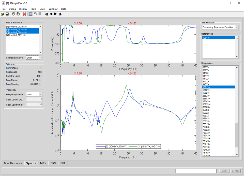
In the Spectra module, frequency-domain measurement functions are read into spVIEW and plotted. The supported function types are FRF, ordinary coherence, multiple coherence, reference coherence, linear spectra, auto-spectra, power spectral density, energy spectral density, reference-response cross-spectra, reference cross-spectra, response cross-spectra, and principal components. Information about the selected datasets and the references and responses in the Coordinate Sieve is displayed in the Data Info panel.
Selecting a plotted line with the mouse pointer and holding down the middle button will highlight that line and its corresponding entry in the plot legend and the name from the legend will be displayed in the message line at the bottom of the window. Selecting an entry in the plot legend with the middle mouse button will toggle highlighting of the corresponding line in the plot axes. The associated line in the other plot axes will also be highlighted, if applicable.
Frequency : Frequency Sieve – When multiple datasets are selected in the Files & Functions list, the Frequency Sieve determines the frequency range for plotting. The Frequency Sieve can be union or intersection, which sieves the frequency ranges of the selected datasets as set operator nomenclature implies, or manual, which allows the frequency range to be specified by the user by entering the Clear Lower and Clear Upper values.
Frequency : Clear Lower & Clear Upper – Enter numeric values in Hertz for the Clear Lower and Clear Upper frequencies. The X limits of the plot axes are set to the Clear Lower and Clear Upper frequencies. There is a context menu on the edit boxes to set the Clear Lower and Clear Upper frequencies according to the Frequency Sieve or to the plot axes X limits. These values can only be entered if the Frequency Sieve is manual.
Plot Function – Select the function type to plot. The available selections are dependent on the measurements (FRF, coherence, auto-spectra, cross-spectra, etc.) contained in the datasets. If multiple datasets are selected in the Files & Functions list, the available Plot Functions are the intersection of the functions types contained in the selected datasets.
When a complex-valued function is plotted, and the complex format is magnitude and phase, there is a context menu on the upper axes y-label ("Phase (deg)") that contains a selection for the "clean phase" option. If "clean phase" is enabled, points where the phase differs by more than 270 degrees from the previous point are not displayed. The "clean phase" option can also be accessed from the Display menu for the Spectra module.
References – Select the references to plot. Use the context menu to select the attributes listed or displayed in the legend, disable selected references, enable all references, sieve by coordinate trace, or plot drive points or reciprocals.
Responses – Select the responses to plot. Use the context menu to select the attributes listed or displayed in the legend, choose an FRF sorting option, disable selected responses, enable all responses, sieve by coordinate trace, find a channel, or to open the Channels dialog.
Selecting Find Channel from the context menu presents an input dialog into which a response coordinate (e.g., 1234X+ or 1234X) or node (e.g., 1234) is entered. Any channel with the specified coordinate or node will be found and plotted. The direction sense (i.e., +/−) is not required and if omitted, any response coordinate with the positive or negative sense of the specified direction will be found.
FRF sorting is intended to rank the responses listed in the Responses listbox from "worst" to "best." The Sort by options are either None, Coherence, or Summary Coherence. Sorting by coherence is based on the average coherence for each response over the plotted frequency range. Sorting by summary coherence is based on the integral of the coherence multiplied by the power spectrum mode indicator function and dividing it by the integral of the power spectrum mode indicator function over the plotted frequency range. Refer to [1] for more information on summary coherence. An FRF sorting value between zero and one is assigned to each response, which is displayed in the plot legend. Sorting by coherence or summary coherence from lowest to highest places responses that are most likely to be nonfunctional at the top of the list. Other reasons for low coherence or summary coherence could be locations with little or no measured response, such as accelerometers on a fixed base. Therefore, it is recommended that the user view these responses manually to determine whether or not the responses are nonfunctional. The FRF sorting options are only applicable if one dataset is selected in the Files & Functions list, and that dataset contains both FRF and coherence functions.
Slide Show – The slide show is an automated means to sequentially plot spectral functions by incrementing one response. All of the selected references are plotted, if applicable (e.g., FRF and cross-spectra). The slide show controls on the toolbar are meant to have similar functionality to the buttons on a DVD player remote control. The slide show can step one response forward or reverse, or play the responses forward or reverse sequentially. In the slide show play mode, the response is automatically incremented on a timed interval. The Slide Show Pause Interval is set in the Preferences dialog.
Tools > Spectra > Send Plot Spectra to IMAT Plot – Sends the plotted spectral functions, truncated according to the Frequency Sieve, to an IMAT plot figure.
Tools > Spectra > Send Plot Spectra to UIPLOT – Sends the plotted spectral functions, truncated according to the Frequency Sieve, to UIPLOT.
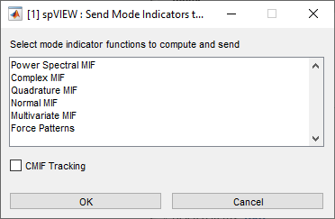
Tools > Spectra > Send Mode Indicators to spVIEW MIFs – Computes mode indicator functions from FRF (or cross spectra for PSMIF and CMIF), sieved according to the Coordinate Sieve and truncated according to the Frequency Sieve, and sends them to the spVIEW MIFs module. A dialog as shown below is presented from which to select the MIFs that are computed and sent. Select the checkbox to enable CMIF tracking. This operation is executed for all datasets selected in the Files & Functions list.
Tools > Spectra > Send Auto Spectra to spVIEW SPL – Sends auto-spectra (and spectra) functions, sieved according to the Coordinate Sieve and truncated according to the Frequency Sieve, to the spVIEW SPL module. The functions sent must have a data type of pressure or sound pressure. This operation is executed for all datasets selected in the Files & Functions list.
Tools > Spectra > Data Type Calculus – Converts displacement, velocity, and acceleration data types. The functions for which this conversion is possible (i.e., channels that have a data type of displacement, velocity, or acceleration) are integrated or differentiated to the selected data type. Channels with other data types are copied unchanged. A new dataset is appended to the Files & Functions list. This operation is executed for all datasets selected in the Files & Functions list.
The spectral functions are integrated using the IMAT integ function as
G = INTEG(F,'freq')
which uses a 1/jw frequency integration. See the help documentation on this function for more detailed information. The spectral functions are differentiated using the IMAT diff function as
G = DIFF(F,'freq')
which uses a jw frequency differentiation. See the help documentation on this function for more detailed information.
Tools > Spectra > Octaves – The auto-spectra and FRF functions are reduced to the 1/N octave bands selected from the submenu using the IMAT octaven function as
G = OCTAVEN(F,N,'rms','silent'[,'ansi'])
See the help documentation on this function for more detailed information. If 1/N is selected from the submenu, an input dialog is presented to define the requested octave bands. Follow the prompts on the dialog to enter the N input argument. A new dataset is appended to the Files & Functions list. This operation is executed for all datasets selected in the Files & Functions list.
Tools > Spectra > Weighting – The auto-spectra functions are A-weighted or C-weighted. A new dataset is appended to the Files & Functions list. This operation is executed for all datasets selected in the Files & Functions list.
Tools > Spectra > Decimation – The spectral functions are decimated using the IMAT decimate function as
G = DECIMATE(F,FACTOR)
See the help documentation on this function for more detailed information. An input dialog is presented to define the input arguments to the function. Follow the prompts on the dialog to enter the FACTOR input argument. A new dataset is appended to the Files & Functions list. This operation is executed for all datasets selected in the Files & Functions list.
Tools > Spectra > Interpolation – The spectral functions are interpolated using the IMAT interp function as
G = INTERP(F,'inc',INCREMENT,'lin',METHOD[,EXTRAPTYPE])
See the help documentation on this function for more detailed information. An input dialog is presented to define the input arguments to the function. Follow the prompts on the dialog to enter the INCREMENT, METHOD, and optional EXTRAPTYPE input arguments. A new dataset is appended to the Files & Functions list. This operation is executed for all datasets selected in the Files & Functions list.
Tools > Spectra > Positive Power Spectra – This tool converts cross spectra functions to positive power spectra (PPS) functions that can be used for operational modal analysis (OMA). A new dataset is appended to the Files & Functions list. This operation is executed for all datasets selected in the Files & Functions list.
Tools > Spectra > Write Spectra Info Structure to CSV File – When the spectral functions are written to an imat_fn in the MATLAB workspace, an accompanying info structure is also created. The imat_fn can be written from the workspace to an AFU or universal file using writeadf or writeunv, respectively. Use this tool to write an info structure to a CSV file. Select the info structure from the variable selection dialog, then select the corresponding AFU file. The CSV file written has same filename, but .info.csv is appended to the extension.