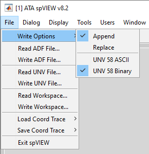
Under the File Menu are the selections to set the write options, read and write datasets, load and save coordinate traces, and exit spVIEW. Each of these features is described below with any details pertinent to a module denoted.
File > Write Options - Select whether to append or replace when writing to files or the MATLAB workspace. Select whether to write ASCII or binary (Dataset 58) Universal files.
File > Read ADF File and File > Read UNV File – Read functions from one or more ADF or Universal files. A file selection dialog is presented from which to browse and select the files to read. Reading multiple files is supported and the contents of each file are read into a new dataset in the Files & Functions list. There is also an icon on the toolbar to read the file type that was last read (default is specified in the INI file). The STOP button on the lower-right corner of the window will stop a file read in progress.
Time Response Module: The ADF file type will most likely be an ATI (time) file, which can contain only time response functions, but it could also be an AFU (function) file, which can contain other types of functions as well as time response functions. The entire file is read, but only the time response functions are retained; all other function types are discarded. The time response functions are verified for consistent attributes (number of elements, sampling type, amplitude units, normalization, and abscissa spacing, minimum, increment, data type, and type qualifier).
Spectra Module: Since the spVIEW Spectra module was originally intended for viewing the spectral function results from spFRF, all the frequency-domain measurement function types generated by spFRF can be read into the spVIEW Spectra module. These function types include FRF, ordinary coherence, multiple coherence, reference coherence, auto-spectra, power spectral density, energy spectral density, reference-response cross-spectra, reference cross-spectra, response cross-spectra, and principal components. In addition, linear spectra functions are also supported. The spectral functions are verified for consistent abscissa attributes (number of elements, sampling type, octave format, and abscissa spacing, minimum, increment, data type, and type qualifier) and ordinate attributes (amplitude units and normalization), as applicable according to the function types. The different types of spectral functions are assumed to have consistent references and responses.
Whenever a spectral functions results file is written from spFRF, a CSV info file is also written to the same folder. The CSV info file has the same filename as the ADF or Universal file, but .info.csv is appended to the extension. This file contains sufficient information to recreate the signal processing results and also the necessary information to reassemble the functions into a consistent set of matrices for each function type similar to that available in the spFRF Results module. If the spFRF results file was generated by appending two or more sets of results into one file, each set of functions is read into a separate dataset in the Files & Functions list.
When the ADF or Universal file of spectral functions was created by spFRF and the CSV info file exists in the same folder, reassembling the function matrices is transparent to the user. However, if a CSV info file is not available, it may be still possible to read at least some of the contents of the file into the Spectra module. If the ADF or Universal file contains only one type of spectral function, spVIEW will attempt to read the contents into a dataset without any further interaction from the user. But if the ADF or Universal file contains more than one type of spectral function, a selection dialog as shown below is presented.
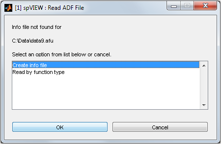
If the Create info file option is selected, a template for a CSV info file is created and opened in the MATLAB Editor as shown below. Edit this file to define the number of references (line 5) and responses (line 6) and measurement functions (line 7) in the associated ADF or Universal file. Then save the file and read the ADF or Universal file again.
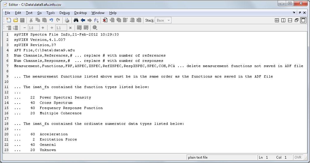
There are some hints about the contents of the file listed at the bottom (lines 11–23). For this example, there are 2 Excitation Force ordinate numerator data types (line 21), which indicates that the number of references is 2. Since there are 40 Frequency Response Function (line 15) and 40 Cross Spectrum (line 14), the number of responses is 40/2 = 20. This is also indicated by the 20 Multiple Coherence (line 16), one for each response. The measurement functions are ASPEC (Power Spectral Density, line 13), XSPEC (Cross Spectrum, line 14), FRF (Frequency Response Function, line 15), and COH (Multiple Coherence, line 16). The measurement functions not contained in the file are deleted from the list in line 7. The measurement functions listed in line 7 must be in the same order as the functions are saved in the file, which is indicated by the list of functions types in lines 13–16, i.e., ASPEC,XSPEC,FRF,COH for this example.
If the Read by function type option is selected, a table dialog as shown below is presented. This table lists some information about the contents of the file, including the types of functions, the number of each type of function, the number of references, and the number of responses. Each block of like function types are grouped and listed in the rows of the table. One or more sets of functions can be selected and read into a separate dataset in the Files & Functions list. As a special case, if only one set of FRF and one set of coherence are selected, both functions types are read into one dataset in the Files & Functions list.

MIFs Module: The entire file is read, but only the mode indicator functions and force patterns are retained; all other function types are discarded. The supported mode indicator functions are the power spectral (PSMIF), complex (CMIF), quadrature (QMIF), normal (NMIF), and multivariate (MMIF). The force patterns computed with MMIF are also supported. The functions are verified for consistent abscissa attributes (number of elements, sampling type, octave format, and abscissa spacing, minimum, increment, data type, and type qualifier).
All of the types of mode indictor functions have a function type attribute of 'Mode Indicator Function' and the force pattern functions have a function type attribute of 'Force Pattern'. When the mode indicator functions are generated by the IMAT functions of the same names, the different types of MIFs are distinguished by their identification line #3 (IDLine3) attribute, as listed below.
|
MIF Type |
IDLine3 Attribute |
| PSMIF | 'N DOF used in PSMIF calculation' |
| CMIF | 'Complex Mode Indicator' |
| QMIF | Quadrature Mode Indicator' |
| NMIF | 'N DOF used in NMIF calculation' |
| MMIF | 'N DOF used in NMIF calculation' |
SRS Module: The entire file is read, but only the SRS functions are retained; all other function types are discarded. The SRS functions are verified for consistent abscissa attributes (number of elements, sampling type, octave format, and abscissa spacing, minimum, increment, data type, and type qualifier) and fully-populated arrays of channels and damping values for all of the SRS function types present in the functions.
SPL Module: The entire file is read, but only spectrum, auto spectrum, and power spectral density functions are retained; all other function types are discarded. The ordinate numerator data type can be either pressure or sound pressure; functions with other ordinate numerator data types are discarded. PSD functions with inconsistent normalization and amplitude units attributes are also discarded. Additionally, functions are discarded that have inconsistent normalization and ordinate numerator type qualifier attributes, non-octave uneven abscissa spacing and 'Units squared/Hz' normalization attributes, or a normalization attribute of 'Units squared sec/Hz'. The remaining functions are verified for consistent abscissa attributes (number of elements, sampling type, octave format, and abscissa spacing, minimum, increment, data type, and type qualifier).
In addition to the standard measurement function types with the attributes defined above, “SPL functions” written from the SPL Module also can be read into the SPL Module.
File > Write ADF File and File > Write UNV File – The functions in the selected datasets in the Files & Functions list can be written to ADF or Universal files, with the append or replace, and ASCII or binary (Universal File Format Dataset 58) options as selected. The functions for multiple selected datasets are all written to one file. A file selection dialog is presented from which to browse and select the file to write. There is also an icon on the toolbar to write the file type that was last written (default is specified in the INI file). The STOP button on the lower-right corner of the window will stop a file write in progress.
Time Response Module: The time response functions for each of the selected Files & Functions are written to an ATI (time), AFU (function), or Universal file. The channels are sieved according to the Coordinate Sieve and only enabled channels are written. The written time response functions are truncated according to the Time Range Sieve.
Spectra Module: The spectra functions (e.g., FRF, Coherence, Auto Spectra, etc.) for each of the selected Files & Functions are written to an AFU (function) or Universal file. The references and responses are sieved according to the Coordinate Sieve and only enabled references and responses are written. The written spectra functions are truncated according to the Frequency Sieve.
Whenever a file is written from the Spectra module, a CSV info file is also written to the same folder. The CSV info file has the same filename as the spectral function file, but .info.csv is appended to the extension. This file contains the necessary information to reassemble the functions in each dataset into a consistent set of matrices for each function type.
MIFs Module: The mode indicator functions and force patterns for each of the selected Files & Functions are written to an AFU (function) or Universal file. The written functions are truncated according to the Frequency Sieve.
SRS Module: The SRS functions for each of the selected Files & Functions are written to an AFU (function) or Universal file. The channels are sieved according to the Coordinate Sieve and only enabled channels are written. The written SRS functions are truncated according to the Frequency Sieve.
SPL Module: The “SPL functions” for each of the selected Files & Functions are written to an AFU (function) or Universal file. The channels are sieved according to the Coordinate Sieve and only enabled channels are written. The written “SPL functions” are truncated according to the Frequency Sieve. An “SPL function” has the following attributes:
|
Attribute |
"SPL Function" |
|
FunctionType |
'Spectrum' |
|
OrdNumDataType |
'Unknown' |
|
OrdNumTypeQual |
'Translation' |
|
OrdNumExpLength |
0 |
|
OrdNumExpForce |
0 |
|
OrdNumExpTemp |
0 |
|
OrdNumExpTime |
0 |
|
OrdinateAxisLab |
'SPL' |
|
OrdinateUnitsLab |
'dB re Pref' |
|
AmplitudeUnits |
'Unknown' |
|
Normalization |
'Unknown' |
For a function with these attributes, the ordinate SPL values (in dB) are not affected by units system conversion on read or write and the default y-label is overridden by the ordinate axis label and ordinate units label.
File > Read Workspace – Read functions from one or more imat_fn in the MATLAB workspace. A variable selection dialog is presented from which to select the imat_fn to read. Reading multiple variables is supported and the contents of each imat_fn are read into a new dataset in the Files & Functions list. There is also an icon on the toolbar.
Time Response Module: The entire imat_fn is read, but only the time response functions are retained; all other function types are discarded. The time response functions are verified for consistent attributes (number of elements, sampling type, amplitude units, normalization, and abscissa spacing, minimum, increment, data type, and type qualifier).
Spectra Module: Since the spVIEW Spectra module was originally intended for viewing the spectral function results from spFRF, all the frequency-domain measurement function types generated by spFRF can be read into the spVIEW Spectra module. These function types include FRF, ordinary coherence, multiple coherence, reference coherence, auto-spectra, power spectral density, energy spectral density, reference-response cross-spectra, reference cross-spectra, response cross-spectra, and principal components. In addition, linear spectra functions are also supported. The spectral functions are verified for consistent abscissa attributes (number of elements, sampling type, octave format, and abscissa spacing, minimum, increment, data type, and type qualifier) and ordinate attributes (amplitude units and normalization), as applicable according to the function types. The different types of spectral functions are assumed to have consistent references and responses.
Whenever a spectral functions results imat_fn is written from spFRF to the MATLAB workspace, an info structure is also created. The info structure has the same variable name as the imat_fn, but with _info appended. This structure contains sufficient information to recreate the signal processing results and also the necessary information to reassemble the functions into a consistent set of matrices for each function type similar to that available in the spFRF Results module. If the spFRF results imat_fn was generated by appending two or more sets of results into one variable, each set of functions is read into a separate dataset in the Files & Functions list.
When the imat_fn of spectral functions was created by spFRF and the info structure exists in the MATLAB workspace, reassembling the function matrices is transparent to the user. However, if an info structure is not available, it may be still possible to read at least some of the contents of the file into the Spectra module. If the imat_fn contains only one type of spectral function, spVIEW will attempt to read the contents into a dataset without any further interaction from the user. But if the imat_fncontains more than one type of spectral function, a selection dialog as shown below is presented.
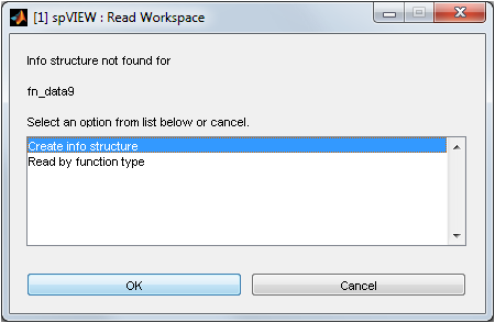
If the Create info structure option is selected, a template for an m-file is created and opened in the MATLAB Editor as shown below. Edit this file to define the number of references (line 9) and responses (line 10) and measurement functions (line 11) in the associated imat_fn. Press Ctrl+Enter to run the m-file and create the info structure in the MATLAB workspace. Then read the imat_fn from the MATLAB workspace again.
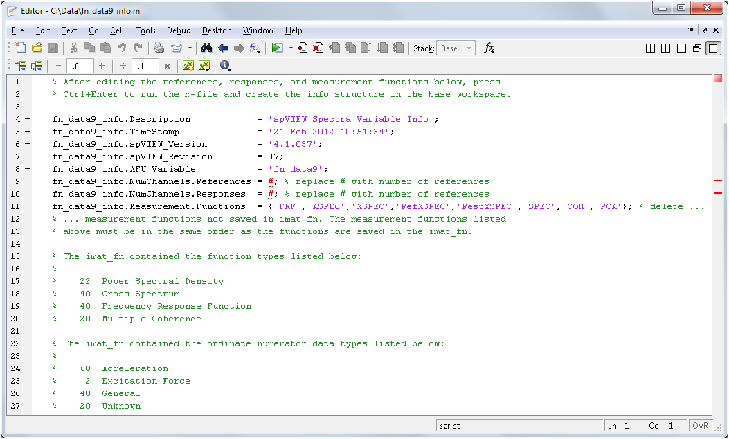
There are some hints about the contents of the imat_fn listed at the bottom (lines 15–27). For this example, there are 2 Excitation Force ordinate numerator data types (line 25), which indicates that the number of references is 2. Since there are 40 Frequency Response Function (line 19) and 40 Cross Spectrum (line 18), the number of responses is 40/2 = 20. This is also indicated by the 20 Multiple Coherence (line 20), one for each response. The measurement functions are ASPEC (Power Spectral Density, line 17), XSPEC (Cross Spectrum, line 18), FRF (Frequency Response Function, line 19), and COH (Multiple Coherence, line 20). The measurement functions not contained in the file are deleted from the list in line 11. The measurement functions listed in line 11 must be in the same order as the functions are saved in the file, which is indicated by the list of functions types in lines 17–20, i.e., ASPEC,XSPEC,FRF,COH for this example.
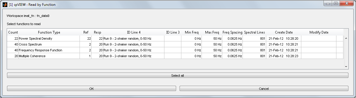
If the Read by function type option is selected, a table dialog as shown below is presented. This table lists some information about the contents of the imat_fn, including the types of functions, the number of each type of function, the number of references, and the number of responses. Each block of like function types are grouped and listed in the rows of the table. One or more sets of functions can be selected and read into a separate dataset in the Files & Functions list. As a special case, if only one set of FRF and one set of coherence are selected, both functions types are read into one dataset in the Files & Functions list.
MIFs Module: The entire imat_fn is read, but only the mode indicator functions and force patterns are retained; all other function types are discarded. The supported mode indicator functions are the power spectral (PSMIF), complex (CMIF), quadrature (QMIF), normal (NMIF), and multivariate (MMIF). The force patterns computed with MMIF are also supported. The functions are verified for consistent abscissa attributes (number of elements, sampling type, octave format, and abscissa spacing, minimum, increment, data type, and type qualifier).
All of the types of mode indictor functions have a function type attribute of 'Mode Indicator Function' and the force pattern functions have a function type attribute of 'Force Pattern'. When the mode indicator functions are generated by the IMAT functions of the same names, the different types of MIFs are distinguished by their identification line #3 (IDLine3) attribute, as listed below.
| MIF Type | IDLine3 Attribute |
| PSMIF | 'N DOF used in PSMIF calculation' |
| CMIF | 'Complex Mode Indicator' |
| QMIF | Quadrature Mode Indicator' |
| NMIF | 'N DOF used in NMIF calculation' |
| MMIF | 'N DOF used in NMIF calculation' |
SRS Module: The entire imat_fn is read,but only the SRS functions are retained; all other function types are discarded. The SRS functions are verified for consistent abscissa attributes (number of elements, sampling type, octave format, and abscissa spacing, minimum, increment, data type, and type qualifier) and fully-populated arrays of channels and damping values for all of the SRS function types present in the functions.
SPL Module: The entire imat_fn is read, but only spectrum, auto spectrum, and power spectral density functions are retained; all other function types are discarded. The ordinate numerator data type can be either pressure or sound pressure; functions with other ordinate numerator data types are discarded. PSD functions with inconsistent normalization and amplitude units attributes are also discarded. Additionally, functions are discarded that have inconsistent normalization and ordinate numerator type qualifier attributes, non-octave uneven abscissa spacing and 'Units squared/Hz' normalization attributes, or a normalization attribute of 'Units squared sec/Hz'. The remaining functions are verified for consistent abscissa attributes (number of elements, sampling type, octave format, and abscissa spacing, minimum, increment, data type, and type qualifier).
In addition to the standard measurement function types with the attributes defined above, “SPL Functions” written from the SPL Module also can be read into the SPL Module.
File > Write Workspace – The functions in the selected datasets in the Files & Functions list can be written to an imat_fn in the MATLAB workspace, with the append or replace option as selected. The functions for multiple selected datasets are all written to one imat_fn. A variable selection dialog is presented from which to select the imat_fn to write. There is also an icon on the toolbar.
Time Response Module: The time response functions for each of the selected Files & Functions are written to an imat_fn in the MATLAB workspace. The channels are sieved according to the Coordinate Sieve and only enabled channels are written. The written time response functions are truncated according to the Time Range Sieve.
Spectra Module: The spectra functions (e.g., FRF, Coherence, Auto Spectra, etc.) for each of the selected Files & Functions are written to an imat_fn in the MATLAB workspace. The references and responses are sieved according to the Coordinate Sieve and only enabled references and responses are written. The written spectra functions are truncated according to the Frequency Sieve.
Whenever an imat_fn is written from the Spectra module, an info structure is also created. The info structure has the same variable name as the imat_fn, but with _info is appended. If multiple datasets are written to the MATLAB workspace, a cell array of info structures is created, with one cell for each of the written datasets. This structure contains the necessary information to reassemble the functions in each dataset into a consistent set of matrices for each function type.
MIFs Module: The mode indicator functions and force patterns for each of the selected Files & Functions are written to an imat_fn in the MATLAB workspace. The written functions are truncated according to the Frequency Sieve.
SRS Module: The SRS functions for each of the selected Files & Functions are written to an imat_fn in the MATLAB workspace. The channels are sieved according to the Coordinate Sieve and only enabled channels are written. The written SRS functions are truncated according to the Frequency Sieve.
SPL Module: The “SPL functions” for each of the selected Files & Functions are written to an imat_fn in the MATLAB workspace. The channels are sieved according to the Coordinate Sieve and only enabled channels are written. The written “SPL functions” are truncated according to the Frequency Sieve. An “SPL function” has the attributes listed above.
File > Load Coordinate Trace – Load coordinate traces from a Universal file or an imat_ctrace (or a cell array of imat_ctraces if more than one) in the MATLAB workspace. A file or variable selection dialog is presented from which to select the file or workspace variable to load. The coordinate traces can be used as filters in the Channels dialog or for sieving from the Channels, Responses, or References listbox context menu. The loaded coordinate traces are appended to any that may have been loaded previously. Use the Clear All menu selection to clear all of the coordinate traces that have been loaded. The coordinate traces loaded while in any module are available in all modules, where applicable.
File > Save Coordinate Trace – Save coordinate traces to a Universal file or an imat_ctrace (or a cell array of imat_ctraces if more than one) in the MATLAB workspace. A file or variable selection dialog is presented from which to select the file or workspace variable to save. The coordinate traces created in the Channels dialog can be saved for future use with this operation.
File > Exit spVIEW – Closes the spVIEW application without a confirmation dialog. Any unwritten datasets will be lost. Closing spVIEW with the [x] button on the upper-right corner of the figure will present a dialog to confirm the user intentions before closing the application.