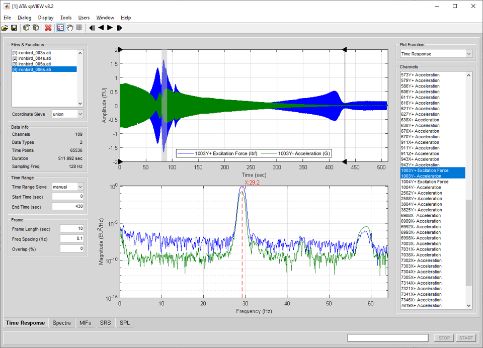
In the Time Response module, time response functions are read into spVIEW and plotted. In addition, properties of the time response (e.g., min, max, mean, and RMS) evaluated for overlapping frames can be computed and plotted. Information about the selected datasets and the channels in the Coordinate Sieve is displayed in the Data Info panel.
The time response functions are plotted in the upper plot axes. Either frame zoom or frame spectra functions are plotted in the lower plot axes. The gray patch in the upper time response plot axes is the frame cursor. Its width is equal to the Frame Length. The Frame Plot is selected from either the Time Response Display menu or the context menu on the lower plot axes x-label. If Frame Plot is Frame Spectra, the spectra of the time segment contained in the frame cursor are plotted in lower plot axes. The Window, Normalization, and Amplitude Units parameters in the Frame Spectra panel are applied to the frame spectra. If Frame Plot is Frame Zoom, the zoomed time segment contained in the frame cursor is plotted in lower plot axes. The Frame Spectra plot is only available if the Plot Function is Time Response.
There is a context menu on the plotted time response functions to bring the selected trace to the front or send it to the back. The context menu on the upper axes has a Frame Cursor Here selection that will move the center of the frame cursor to the mouse pointer position. On this axes context menu and also on the Time Response Display menu is a Frame Cursor selection to toggle the visibility of the frame cursor on and off. There is a context menu on the frame cursor to select the cursor color and to stretch the frame cursor. To stretch the frame cursor to the right, select Stretch Right from the frame cursor context menu and then click on the cursor patch. The left edge of the cursor is anchored and the right edge moves with the mouse pointer. The Stretch Left operation anchors the right edge of the frame cursor and the left edge moves with the mouse pointer.
Selecting a plotted line with the mouse pointer and holding down the middle button will highlight that line and its corresponding entry in the plot legend and the name from the legend will be displayed in the message line at the bottom of the window. Selecting an entry in the plot legend with the middle mouse button will toggle highlighting of the corresponding line in the plot axes. The associated line in the other plot axes will also be highlighted, if applicable.
Time Range : Time Range Sieve – When multiple datasets are selected in the Files & Functions list, the Time Range Sieve determines the time range for plotting. The Time Range Sieve can be union or intersection, which sieves the time ranges of the selected datasets as set operator nomenclature implies, or manual, which allows the time range to be specified by the user by entering the Start Time and End Time values.
Time Range : Start Time & End Time – If the Time Range Sieve is manual, enter the start and end limits of the Time Range for plotting. These values can also be set using the two Time Range cursors in the upper plot axes. There is a context menu on the edit boxes from which to set the Time Range according to the Time Range Sieve, or to the upper plot axes X limits or the frame cursor. The upper plot axes X limits can also be set to the Time Range from this context menu.
Frame : Frame Length & Frequency Spacing – Enter numeric values for the Frame Length in seconds or Frequency Spacing in Hertz. According to Rayleigh’s Criterion, these two parameters are reciprocals of one another.
Frame : Overlap – Enter a numeric value for the Overlap as a percentage of the Frame Length. This parameter is used for processing properties of time response functions (e.g., min, max, mean, and RMS) for overlapping frames, which can then be plotted.
Frame Spectra : Window – Select the type of Window to apply for the frame spectra. The choices are uniform (aka, 'boxcar', 'rectangular', or 'none'), hanning broad, hanning narrow, hamming, flattop, half sine, or exponential. The exponential window parameters are entered in the Windowing dialog shown below, which is opened from the Dialog menu or from the context menu on the Window popup menu.
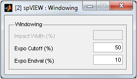
The exponential window decay is defined by Expo Cutoff and Expo Endval. The exponential window starts at a value of 1 at time 0, and Expo Cutoff and Expo Endval define a second point on the exponential decay, as shown below.
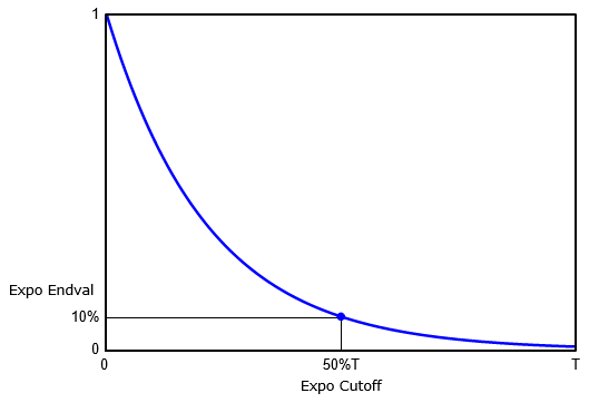
Expo Cutoff is entered as a percentage of the time frame length (T) and Expo Endval is entered as a percentage of unity. The exponential window time constant is computed such that the window decays from a value of 1 at time 0 to the value defined by Expo Endval (y-value) at the time in the frame length defined by Expo Cutoff (x-value).
Frame Spectra : Normalization – Select the Normalization attribute for the frame spectra functions, as either EU for spectra, EU^2 for power spectra, EU2/Hz for power spectral density (PSD), or EU2s/Hz for energy spectral density (ESD).
Frame Spectra : Amplitude Units – Select the Amplitude Units attribute for the frame spectra functions, as either rms, peak, or half-peak.
Frame Spectra : Frequency Sieve – When multiple datasets are selected in the Files & Functions list, the Frequency Sieve determines the frequency range for plotting. The Frequency Sieve can be union or intersection, which sieves the frequency ranges of the selected datasets as set operator nomenclature implies, or manual, which allows the frequency range to be specified by the user by entering the Clear Lower and Clear Upper values.
Frame Spectra : Clear Lower & Clear Upper – Enter numeric values in Hertz for the Clear Lower and Clear Upper frequencies. The X limits of the lower frame spectra plot axes are set to the Clear Lower and Clear Upper frequencies. There is a context menu on the edit boxes to set the Clear Lower and Clear Upper frequencies to the full Nyquist bandwidth (0 - Nyquist) , the customary alias-protected bandwidth (0 – Span), or the lower plot axes X limits. If multiple datasets are selected, the sampling frequency is the maximum of the selected datasets.
Plot Function – Select the function type to plot. In addition to Time Response, there a number of frame metric plots available. These frame metric plots are generated by processing the time response functions in overlapped frames. Dynamic RMS is the RMS of the signal after subtracting the mean, that is, the RMS of the dynamic part of the signal. Positive and negative RMS is the RMS of the positive and negative parts of the signal, respectively. Channel Overview plots the minimum, maximum, mean, ±RMS, positive RMS, and negative RMS for one channel. Frame SPL is applicable only to channels with a data type of pressure or sound pressure. The STOP button will stop the frame processing in progress. If the Plot Function is anything other than Time Response, the Frame Spectra plot is not available. When plotting the channel overview or a frame metric, the time response of the zoomed time segment contained in the frame cursor is plotted in lower plot axes.
Channels – Select the channels to plot. Use the context menu to select the attributes listed or displayed in the legend, choose a sorting option, disable selected channels, enable all channels, sieve by coordinate trace, find a channel, or open the Channels dialog.
Selecting Find Channel from the context menu presents an input dialog into which a response coordinate (e.g., 1234X+ or 1234X) or node (e.g., 1234) is entered. Any channel with the specified coordinate or node will be found and plotted. The direction sense (i.e., +/−) is not required and if omitted, any response coordinate with the positive or negative sense of the specified direction will be found.
The sorting options are intended to rank the channels by some data quality metric from "worst" to "best." The Sort by options are None, Dynamic RMS, and Dynamic Crest Factor. The dynamic RMS is the RMS of the signal after subtracting the mean, that is, the RMS of the dynamic part of the signal. The dynamic crest factor is the ratio of the dynamic peak to the dynamic RMS, where the dynamic peak is the peak of the signal after subtracting the mean. Sorting by dynamic RMS sorts the channels from lowest to highest. Putting the channels with the smallest response at the top of the list should aid in finding nonfunctional channels. Sorting by dynamic crest factor sorts the channels from highest to lowest. This data quality metric is often useful to find responses that contain spurious glitches. These sorting options are only available when only one dataset is selected in the Files & Functions list.
Slide Show – The slide show is an automated means to sequentially plot time response functions by incrementing one channel. The slide show controls on the toolbar are meant to have similar functionality to the buttons on a DVD player remote control. The slide show can step one channel forward or reverse, or play the channels forward or reverse sequentially. In the slide show play mode, the channel is automatically incremented on a timed interval. The Slide Show Pause Interval is set in Preferences dialog.
Tools > Time Response > Send Plot Channels to IMAT Plot – Sends the plotted time response functions in the upper plot axes, truncated according to the Time Range Sieve, to an IMAT plot figure.
Tools > Time Response > Send Plot Channels to UIPLOT – Sends the plotted time response functions in the upper plot axes, truncated according to the Time Range Sieve, to UIPLOT.
Tools > Time Response > Send Frame Zoom to IMAT Plot – Sends the plotted time response functions in the lower plot axes to an IMAT plot figure. This tool is only available when the Frame Plot is Frame Zoom.
Tools > Time Response > Send Frame Zoom to UIPLOT – Sends the plotted time response functions in the lower plot axes to UIPLOT. This tool is only available when the Frame Plot is Frame Zoom.
Tools > Time Response > Send Frame Spectra to IMAT Plot – Sends the plotted frame spectra in the lower plot axes, truncated according to the Frequency Sieve, to an IMAT plot figure.
Tools > Time Response > Send Frame Spectra to UIPLOT – Sends the plotted frame spectra in the lower plot axes, truncated according to the Frequency Sieve, to UIPLOT.
Tools > Time Response > Send Frame Spectra to spVIEW Spectra – Sends the plotted frame spectra in lower plot axes, truncated according to the Frequency Sieve, to the spVIEW Spectra module.
Tools > Time Response > Data Type Calculus – Converts displacement, velocity, and acceleration data types. The channels for which this conversion is possible (i.e., channels that have a data type of displacement, velocity, or acceleration) are integrated or differentiated to the selected data type. Channels with other data types are copied unchanged. A new dataset is appended to the Files & Functions list. This operation is executed for all datasets selected in the Files & Functions list.
The time response functions are integrated using the IMAT integ function as
G = INTEG(F)
which uses a simple trapezoidal rule integration. See the help documentation on this function for more detailed information. The time response functions are differentiated using the IMAT diff function as
G = DIFF(F)
which uses a simple dy/dx differentiation. See the help documentation on this function for more detailed information.
Tools > Time Response > Signal Processing – This tools menu has a number of signal processing operations. After performing the signal processing operation, a new dataset is appended to the Files & Functions list. This operation is executed for all datasets selected in the Files & Functions list.
> Truncate to Time Range – The time response functions are truncated according to the Time Range Sieve, which is defined by the values specified by the Start Time and End Time.
> Resample – The time response functions are resampled using the MATLAB resample function as
Y = RESAMPLE(X,P,Q,N,BTA)
See the help documentation on this function for more detailed information. An input dialog is presented to define the input arguments to the function. Follow the prompts on the dialog to enter numeric values for the P, N, and BTA input arguments.
> Decimate – The time response functions are decimated using the IMAT decimate function as
G = DECIMATE(F,FACTOR,METHOD[,ARGS])
See the help documentation on this function for more detailed information. An input dialog is presented to define the input arguments to the function. Follow the prompts on the dialog to enter the FACTOR, METHOD and optional ARGS input arguments.
> Interpolate – The time response functions are interpolated using the IMAT interp function as
G = INTERP(F,'inc',INCREMENT,'lin',METHOD[,EXTRAPTYPE])
See the help documentation on this function for more detailed information. An input dialog is presented to define the input arguments to the function. Follow the prompts on the dialog to enter the INCREMENT, METHOD, and optional EXTRAPTYPE input arguments.
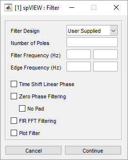
> Filter – A dialog is presented as an interface to the IMAT filteri, filterf, and filteru functions. The Filter Design can be selected for infinite impulse response (IIR) and finite impulse response (FIR) lowpass, highpass, bandpass, and bandstop filters and also user-supplied filters. Some of the filtering functionality requires the MATLAB Signal Processing toolbox.
For IIR filter designs, the time response functions are filtered using the IMAT filteri function as
OUT = FILTERI(IN,TYPE,WP,NPOLES[,'silent'])
where TYPE specifies the type of IIR filterfilter (highpass, lowpass, bandpass, or bandstop), WPis the filter frequency, and NPOLES is the number of poles. See the help documentation on this function for more detailed information.
For FIR filter designs, the time response functions are filtered using the IMAT filterf function as
OUT = FILTERF(IN,TYPE,WP,[,WS][,'silent'][,'nopad'])
where TYPE specifies the type of FIR filter (highpass, lowpass, bandpass, or bandstop), WP is the filter frequency, and WS the edge frequency (optional, leave empty for the default). See the help documentation on this function for more detailed information.
For user-supplied filter designs, the time response functions are filtered using the IMAT filteru function as
OUT = FILTERU(IN,F1[,F2,F3,F4][,'zerophase'][,'firfft'][,'silent'])
where F1[,F2,F3,F4]define the filter. The supported filter forms are: IIR transfer function numerator and denominator arrays (B,A); FIR transfer function numerator array (B); zero, pole, and gain arrays (Z,P,K); state-space arrays (A,B,C,D); second order sections array (SOS); digitalFilterobject; dfilt object. A variable selection dialog is presented from which to select the filter definition array(s) or object. The filter form can be determined from the number and properties of the selected variables except for the zero-pole-gain form. For this filter form, the variable name of the array containing the zeros must begin with 'Z' or 'z' and the variable name of the array containing the poles must begin with 'P' or 'p'. See the help documentation on this function for more detailed information. If the Time Shift Linear Phase option is selected, the abscissa minimum attribute of the filtered time response functions is adjusted to account for the constant group delay of a linear phase filter.
> Smooth – A dialog is presented as an interface to the MATLAB (smoothdata function. See the help documentation on this function for more detailed information. Some of the data smoothing functionality requires the MATLAB Signal Processing toolbox.

> Remove DC Bias – The mean of the time response functions between the two Time Range cursors is subtracted from the time response functions to remove the DC bias.
Tools > Time Response > Frame Metrics – Properties of the time response functions processed in overlapped frames are referred to as “frame metrics.” These functions, which can be selected as a Plot Function, can also be read into a dataset in the Files & Functions list using this tool. This operation is executed for all datasets selected in the Files & Functions list.
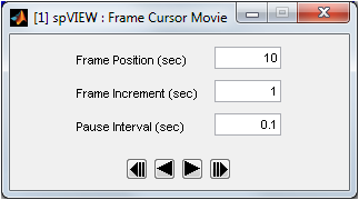
Tools > Time Response > Frame Cursor Movie – This tool is used to step the frame cursor sequentially across the Time Range at a constant increment and rate. The frame spectra or frame zoom in the lower plot axes are updated at each increment of the frame cursor. Enter the Frame Position, in seconds, and the left edge of the frame cursor will move to that time position. Enter the Frame Increment, in seconds, to specify how far the frame cursor moves for each increment. Enter the Pause Interval, in seconds, to specify how long the frame cursor pauses before stepping to the next increment. The controls at the bottom of the GUI are meant to have similar functionality to the buttons on a DVD player remote control. The frame cursor movie can step one increment forward or reverse, or play the increments forward or reverse sequentially. In the play mode, the position of the frame cursor is automatically incremented on a timed interval. There is a context menu on the Frame Position edit box to refresh its value to the current left edge time position of the frame cursor. This will synchronize the Frame Cursor Movie GUI with the current position of the frame cursor if it had been moved manually after the Frame Cursor Movie GUI was opened. The frame cursor movie will stop when it reaches either edge of the Time Range.
Tools > Time Response > Read by Measurement Run – If more than one measurement run (i.e., data acquisition start) is stored to the same ADF file, each data acquisition start increments the measurement run attribute of the records stored to the file. A file selection dialog is presented from which to browse and select the file to read. An imat_fn in the MATLAB workspace can also be read by measurement run, in which case a variable selection dialog is presented from which to select the imat_fn to read. The time response functions associated with each measurement run are read into a separate dataset in the Files & Functions list.
Tools > Time Response > Read by Number Elements – All of the functions read into a dataset must have consistent abscissa attributes, including the number of elements (i.e., time points). A file selection dialog is presented from which to browse and select the file to read. An imat_fnin the MATLAB workspace can also be read by number elements, in which case a variable selection dialog is presented from which to select the imat_fn to read. The time response functions having the same number of elements are read into a separate dataset in the Files & Functions list.